Displacement Control Analysis

Displacement control analysis is a new capability available exclusively in the SG-X solver. It provides an alternative to the conventional load controlled nonlinear analysis, and is particularly valuable for structures that exhibit snap through, post buckling, or softening behaviour where load controlled methods may fail to converge.

What is Displacement Control?

In a standard nonlinear analysis, the applied loads are increased incrementally and the solver computes the corresponding displacements at each step. However, in displacement control analysis, the approach is reversed: a target displacement is prescribed at a specific degree of freedom (the control DOF), and the solver computes the load factor required to achieve that displacement.

At each load step, all applied loads are multiplied by a scalar load factor that is automatically computed by the solver so that the displacement at the control DOF matches the prescribed target value. This allows the solver to trace the full load versus displacement path, including regions where the load may decrease, something that load controlled methods cannot capture.

When to Use Displacement Control

Displacement control analysis is recommended in the following scenarios:

Snap through behaviour. Structures that exhibit a sudden jump in displacement under a critical load level.
Post buckling analysis. Tracing the structural response beyond the buckling point, where the load versus displacement curve may have a descending branch.
Softening behaviour. Structures with material or geometric softening where the load capacity decreases with increasing deformation.
Collapse analysis. Determining the ultimate capacity and failure mode of a structure by pushing it to large displacements.

Setting Up Displacement Control in SPACE GASS

To enable displacement control, tick Perform displacement control analysis in the Displacement Control Analysis (SG-X Only) section at the bottom of the nonlinear analysis dialog. You need to specify the following parameters:

Node. The node at which the displacement is controlled.
Displacement. The target displacement to be achieved at the control node, in the model’s displacement units (e.g. mm).
Axis. The direction of the controlled displacement (X Axis, Y Axis, or Z Axis).

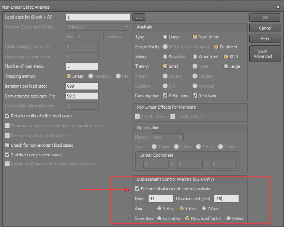
The solver will then automatically adjust the load factor at each step so that the displacement at the specified node and direction reaches the prescribed target value progressively over the load steps defined in the analysis settings.

The Number of load steps should be set to more than 1: typically 10 to 20 steps is recommended. The more steps used, the smoother and more detailed the load versus displacement curve will be, but at the cost of increased computing time.

In the example shown above, Node 41 is chosen as the control node and its target displacement is entered as −25 mm with the Y Axis selected. The negative sign means that Node 41 is driven 25 mm in the direction opposite to the positive Y axis. As the analysis proceeds, the solver computes the load factor required to reach each successive displacement target at Node 41, so it captures the load factor versus displacement response of that node. Here the Save step option is set to Max. load factor, so the saved results correspond to the peak of that curve.

Saving Analysis Results

In the current version of SPACE GASS, only one step of the nonlinear analysis results is saved at a time. For displacement control analysis, the Save step option provides three choices:

Last step. Saves the results at the final load step, where the applied force corresponds to the target displacement.
Max. load factor. The program automatically determines the step at which the load factor is at its maximum. This corresponds to the peak of the load versus displacement curve and represents the maximum load carrying capacity of the structure.
Select. Allows the user to select any step from the load versus displacement curve, providing full flexibility to examine the structural response at any point along the loading path.

Example: Simply Supported Beam

As an example, consider a simply supported beam modelled with shell elements and loaded with a unit load of 1 kN. The objective is to obtain the load versus displacement curve at the mid span node: specifically, the node at the intersection between the web and the flange at mid span.

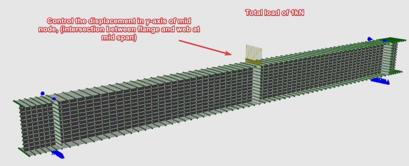
By enabling displacement control and specifying this node as the control node, the solver incrementally increases the displacement at that location. In this model the control node is the mid span node at the top flange, and its displacement is controlled to a target of −25 mm along the Y axis: the negative sign drives the node 25 mm in the direction opposite to the positive Y axis, matching the direction in which the beam deflects under the applied load. These are the settings shown earlier, where the control node is entered as Node 41. At each step, the solver computes the corresponding load factor, effectively tracing the full load versus displacement curve. This provides valuable insight into the structural behaviour, including the elastic, yielding, and post yield response of the beam.

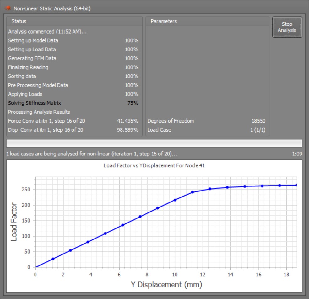
During the analysis, a real time load versus displacement curve is plotted in the analysis progress window, allowing users to monitor the structural response as each load step is solved.

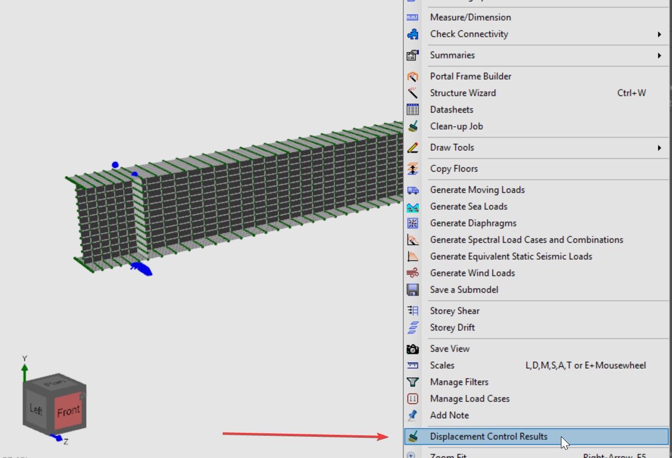
Once the analysis has been completed, the load versus displacement curve can be accessed through the right click context menu by selecting Displacement Control Results.

In this example, the simply supported beam was analysed with nonlinear geometry turned off and nonlinear material turned on. The resulting load versus displacement curve is shown below.

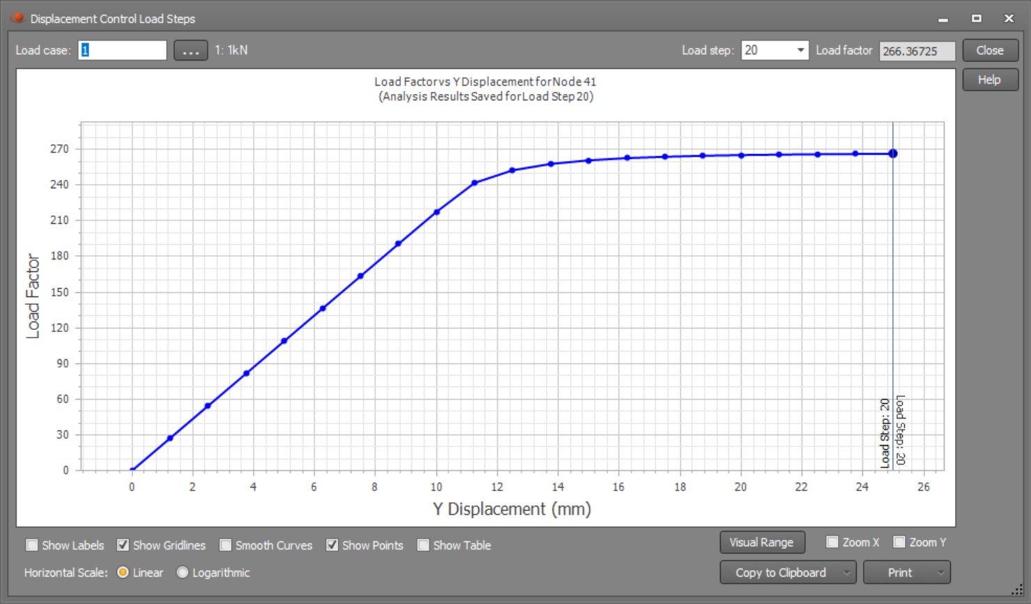
The curve clearly shows that the maximum load factor is approximately 263, which corresponds to a total load of 263 kN (since the applied unit load is 1 kN). The beam displaces around 16 mm before it begins to lose stiffness, indicating the onset of material yielding. Beyond this point, the curve flattens as the beam undergoes plastic deformation with diminishing load carrying capacity.