Non-linear Material for Shell elements
One of the most significant new capabilities introduced by SG-X is support for nonlinear material behaviour in plate/shell elements. The previous solvers (Paradise and Wavefront) only support nonlinear geometry for shell elements. With SG-X, engineers can now perform analyses that account for both geometric and material non-linearity, enabling more realistic modelling of structures where yielding, plasticity, or other material nonlinear effects are important.
Enabling Non-linear Material
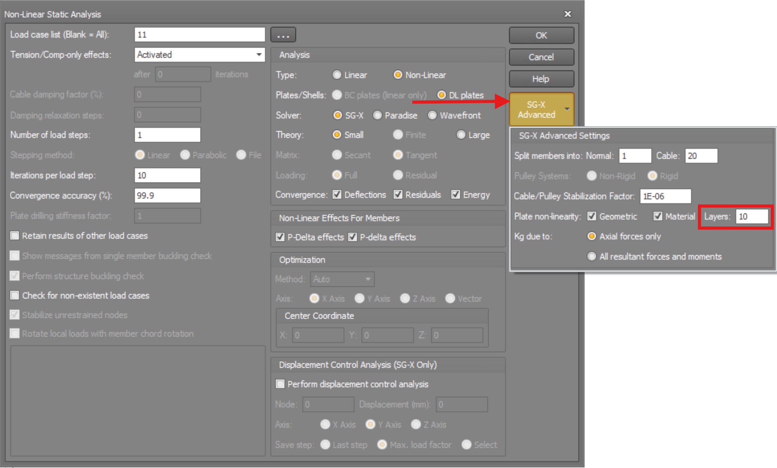
By default, when running a non-linear analysis with SG-X, nonlinear geometry is enabled and nonlinear material is disabled. To activate non-linear material behaviour for shell elements, open the SG-X Advanced Settings panel in the analysis dialog and enable the Material option under Plate non-linearity.
The settings panel also includes a smooth stresses over all plates option, intended to improve the continuity of stress results across adjacent shell elements. In the current release this option is not yet active for SG-X and is reserved for a future update.
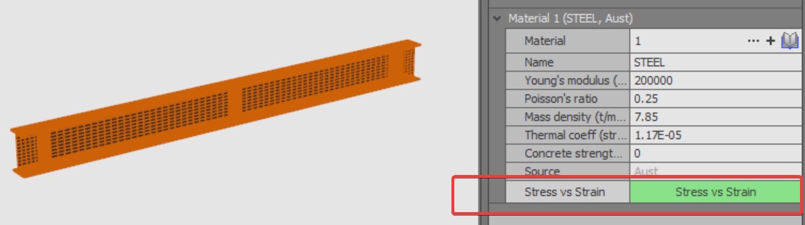
 When non-linear materials is ticked, all materials used by the plate elements must have a stress strain curve
Through Thickness Integration: Number of Layers
When non-linear material is enabled, the SG-X solver uses a layered shell approach to capture material non-linearity through the thickness of each shell element. The shell cross section is divided into a number of layers, and at each layer the stress and strain state is evaluated independently. This allows plasticity to develop progressively from the outer fibres inward, providing a realistic representation of yielding through the thickness.
The Number of Layers parameter (visible in the SG-X Advanced Settings panel) controls how many integration layers are used through the thickness. The default value is 10, which provides a good balance between accuracy and computational cost for most practical applications.
Key points about the layered approach:
- Each layer uses a von Mises elastoplastic constitutive law with isotropic hardening, evaluated at integration points through the thickness of the layer.
- Stresses are computed independently at each layer and can vary non-linearly through the thickness, unlike the linear distribution assumed in elastic analysis.
- A higher number of layers provides finer resolution of the stress gradient through the thickness, which can be important for capturing the onset and spread of plasticity more accurately.
- For most structural engineering applications, the default of 10 layers is sufficient. Increasing this value may be warranted for thick shells or when highly detailed stress distributions through the thickness are required.
For shell elements to be considered for nonlinear material analysis, a Stress vs Strain table must be defined for the material associated with the shell elements. This table defines the elastoplastic material curve used by the solver at each integration layer. If the table is missing, the analysis will not run: SG-X stops with a validation error identifying the material concerned.
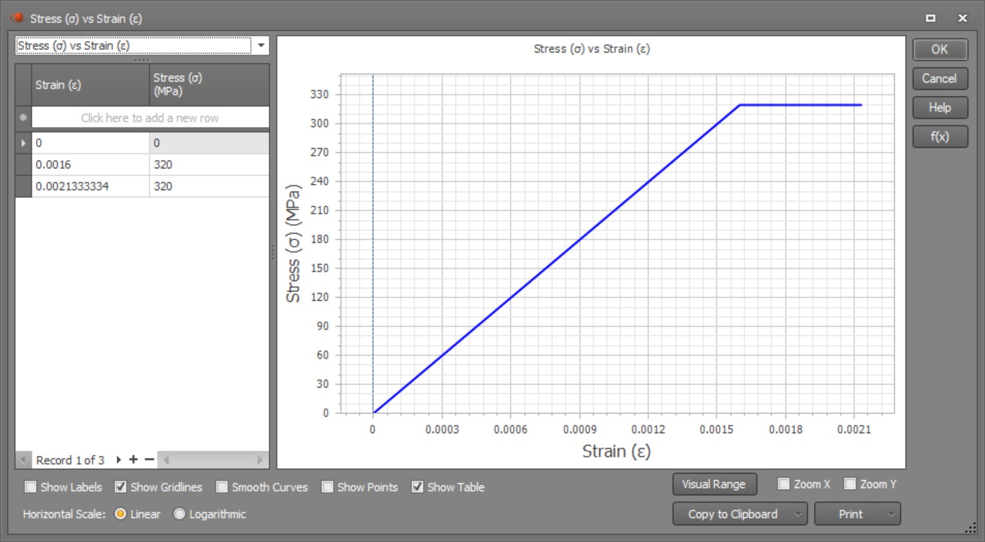
The figure below shows a typical stress strain curve for an elastic perfectly plastic steel material model, which is commonly used for steel structures. The curve shows a linear elastic region up to the yield stress, followed by a horizontal plateau indicating perfectly plastic behaviour with no strain hardening. Note that the yield stress varies depending on the steel grade: the values shown are for illustration purposes only.
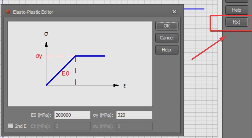
A quick way to define the stress strain curve is via the Elastoplastic Editor, accessible by clicking the f(x) button in the Stress vs Strain dialog. The editor allows you to specify the Young’s modulus (E0) and yield stress (σy) to automatically generate the curve. Alternatively, users can directly enter individual stress strain data points in the table for more complex material models.