SG-X Advanced Settings

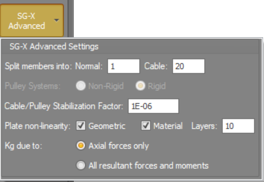
The SG-X Advanced button (on the analysis dialog) opens a small panel of options that control how the SG-X engine builds and solves the finite element model. They do not change your structure. They change the internal discretisation, the element formulations, and the numerical strategy the solver uses to reach a solution. This topic explains each item so you can decide when the defaults are appropriate and when to change them.

Refer Quick Reference

Split members into: Normal and Cable

What it is. SG-X does not necessarily analyse each of your members as a single finite element.
Before solving, it can internally sub-divide a member into several shorter elements joined end to end. These two
fields set how many elements each member is divided into: one count for ordinary (Normal)
members and a separate count for Cable members.

What it does. Each internal element carries only a simple straight line displacement field between its two end nodes, so a single element cannot bend or curve within its own length. Dividing a member into several elements creates interior nodes that are free to move, so the chain of straight segments can approximate a curved deflected shape. More segments give a finer approximation of that shape, and they also give more result points along the member.

Defaults. Normal = 1 , Cable = 20

Why the two defaults differ so much.

Normal members: are solved with a beam element that already includes full bending stiffness. One element per member captures the primary flexural behaviour correctly, so the default is 1. You only raise this when you want to resolve deflection or member buckling shapes in finer detail along the length of a single member.
Cable members: are solved as axial elements that carry tension along their axis and have no bending stiffness of their own. A single straight cable element can therefore only ever be a straight line and cannot represent the sag of a real cable. The curved catenary profile of a cable under its own weight or lateral load is produced only by the polygon of many short segments, each free to find its own tension direction. Around 20 segments gives a smooth, realistic sagging shape, which is why the cable default is much higher.

$image\ebx_-1773499217.gif$ Truss members are always solved as a single element regardless of this setting. A truss element is a straight member carrying axial force only between two pins, so subdividing it would add nothing.

$image\ebx_-1773499217.gif$ The number of elements is a direct multiplier on model size. Splitting a member into N elements adds N −1 interior nodes and that many extra degrees of freedom. Higher counts improve shape accuracy at the cost of solution time and memory, so raise them only where the extra detail matters.

Pulley Systems: Rigid and Non-Rigid

What it is. A pulley system in SG-X is a single rope threaded through a chain of nodes (the wheels) and anchored at its two ends. In both options the rope slides frictionlessly over the intermediate wheels, so the tension is the same all along the rope. This setting does not change that. What it changes is the way the rope itself resists load, that is, its stiffness law.

Rigid (the default).

The rope is given a constant linear axial stiffness and resists both tension and compression.
Because its stiffness never drops away, the rope always stays taut in the numerical model and cannot go slack.
This is the stable, well behaved choice and it converges reliably. The word "rigid" here refers to the rope using a fixed stiffness law, not to any rigid body constraint.

Non-Rigid.

The rope is given a tension only law: it develops its full axial stiffness when pulled in tension, but has zero stiffness when it would be pushed, so it goes slack and carries nothing in compression.
This is the physically realistic behaviour of a real rope or chain, which cannot push.
Because the stiffness switches on and off with the sign of the force, this option is more demanding on the solver and can be slower or harder to converge. It is intended for use with the non-linear solver.

Which one to use. Use Rigid for general modelling and for the most reliable convergence. Choose Non-Rigid when it is important that a rope in a pulley system is allowed to go genuinely slack (carry no force) rather than being held with a small artificial stiffness.

Cable/Pulley Stabilization Factor

What it is. A very small number (default 1 ×10−6) that keeps the solution numerically stable for members that carry axial force only: cables and rigid pulley ropes.

Why it is needed. A cable element has no stiffness across its axis of its own. All of its sideways stiffness comes from the tension it is carrying: a taut string is stiff sideways, a slack string is not. When such a member loses its tension and goes slack, its sideways stiffness falls to zero. If that happens the overall stiffness of the model can become singular, the solver meets a zero on the diagonal, and the analysis stops.

What it does. The factor sets a tiny floor on the force each of these members is assumed to carry, equal to the factor multiplied by the member axial stiffness (EA). That floor guarantees a small residual sideways stiffness at all times, so the model never becomes singular while the solver is iterating. The moment a member picks up more real tension than this floor, the floor is ignored and has no further effect.

$image\ebx_-1773499217.gif$ minimum stabilising force = factor × EA (default factor=1×10−6)

$image\ebx_-1773499217.gif$ Because the default is only one part in a million of the member axial stiffness, the stabilising force is far too small to affect real results once the structure is loaded. It is a convergence aid for the early iterations and for members that would otherwise be completely slack, not a real member force.

$image\ebx_-1773499217.gif$ The factor must be a positive, non-zero value. SG-X will not run a model that contains a cable, truss, or pulley member if this is set to zero. If you see slack cables preventing convergence, a modest increase can help stability, at the cost of introducing a slightly larger artificial force.

Plate non-linearity: Geometric, Material and Layers

These options control how plate elements behave in a non-linear analysis. The Geometric and Material checkboxes are fully independent of each other. You may tick either, both, or neither, and all four combinations are valid.

$image\ebx_-1773499217.gif$ Geometric unticked, and can you mix? If Geometric is unticked, the plate is treated as geometrically linear (small deflection). And yes, the two boxes are independent, so you can absolutely have a geometrically linear plate that still uses a non-linear material. Ticking Material does not force Geometric on, and ticking Geometric does not force Material on.

1. Geometric

Ticked. The plate uses a large deflection formulation. Equilibrium is enforced on the deformed shape of the plate, and the plate stiffness is updated as it deflects and rotates. This is what captures the genuinely nonlinear effects of large deformation: membrane stress stiffening of a laterally loaded plate (a taut plate stiffens as it deflects), post buckling behaviour, and snap through.
Unticked. The plate uses the standard small deflection formulation. Its stiffness is constant and is never updated as the plate deflects. This is the classic linear plate behaviour and is correct whenever deflections are small relative to the plate thickness.

$image\ebx_-1773499217.gif$ Both formulations already include in plane (membrane) action and bending. The Geometric option is not what turns membrane behaviour on. It is what turns on the large deflection treatment in which the stiffness follows the deformed geometry. Note also that this plate option is separate from the displacement theory chosen for frame members: plates have their own geometric non-linearity switch here.

2. Material

Ticked. The plate uses a nonlinear material, defined by the stress and strain curve of the plate material rather than a single elastic modulus. This lets the plate yield and carry load into the plastic range. This behaviour is covered in full in the nonlinear material topic, so only a short description is given here. A stress and strain table must be defined for the plate material, otherwise the analysis cannot run.

$image\ebx_-1773499217.gif$ When this is ticked, all materials used by the plate elements must have a stress strain curve

3. Layers

What it is. When Material is ticked, the plate thickness is sliced into this many equal layers stacked through the thickness. The nonlinear material law is evaluated separately in each layer.

What it does. Under bending, the stress varies across the thickness of a plate, so yielding starts at the outer surfaces and the yielded zone spreads inward as the load rises. The number of layers is the number of sampling stations the solver uses to follow that pattern across the thickness. A small number of layers gives only a coarse picture of the spread of yielding. More layers (the default is 10) give a smoother and more accurate representation of progressive yielding and of the plate bending stiffness once part of the section has yielded.

$image\ebx_-1773499217.gif$ More layers means more accuracy but more work: the nonlinear material law is evaluated in every layer, on every iteration, of every load step. Ten layers is a sensible default. Increase it only when you need very fine detail of the plastic behaviour through the thickness.

K_g due to: Axial forces only, or All resultant forces and moments

What it is. K_g is the geometric stiffness matrix (also called the stress stiffness matrix). It is the part of the model stiffness that represents how the forces already in the structure change its stiffness against further deformation: a member in tension is stiffened sideways, a member in compression is softened and can eventually buckle. This setting controls which internal actions are used to build K_g. It applies to non-linear static analysis and to buckling analysis.

Axial forces only (the default).

K_g is built from each member axial force alone.
This is the classic and robust basis for column and frame buckling and for second order (P ∆) analysis, where the destabilising effect is the axial compression acting through the sideways deflection.
It is efficient and well behaved, and it deliberately leaves out the more exotic instability modes that may not occur in a real structure because of the way its joints are detailed.

All resultant forces and moments.

K_g is built from the complete set of internal actions in each member: axial force plus bending moments, shear, and torsion.
This is a fuller, higher order geometric stiffness that captures instabilities driven by bending and torsion, not only by axial load. The most important example is lateral torsional buckling of beams and beam columns, and flexural torsional modes of slender or open sections.
It is more complete and can predict lower, more conservative critical loads for those cases, but it introduces extra buckling modes and is more demanding on the solver, so it can converge more slowly.

Which one to use: Leave the setting on Axial forces only for ordinary column and frame buckling and for general second order analysis. It is the efficient, reliable default. Switch to All resultant forces and moments when the stability you care about is driven by bending or torsion, most notably lateral torsional buckling of unrestrained beams and flexural torsional buckling of slender open sections.

Quick Reference

Setting	Default	Purpose
Split members: Normal	1	Elements per ordinary member. One is enough because beam elements include bending. Raise for finer detail along a member.
Split members: Cable	20	Elements per cable. Many are needed so the straight segments can form the curved sagging (catenary) shape.
Pulley Systems	Rigid	Rope stiffness law. Rigid: constant stiffness, always taut, stable. Non-Rigid: tension only, can go slack, realistic but harder to solve.
Stabilization Factor	1 ×10⁻⁶	Tiny floor force on cables, trusses and rigid pulleys so they keep a small sideways stiffness and the solver stays stable when they go slack. Must be greater than zero.
Plate: Geometric	Off	On: large deflection plates (membrane stiffening, post buckling). Off: small deflection (linear geometry).
Plate: Material	Off	On: nonlinear (yielding) material for plates. Independent of Geometric.
Plate: Layers	10	Slices through the plate thickness used to follow the spread of yielding. More layers, more accuracy, more cost.
K_g due to	Axial forces only	Actions used to build the geometric stiffness. Axial only: standard column and frame buckling. All forces and moments: also captures lateral torsional and flexural torsional buckling.
Convergence accuracy	99.9%	Iteration tolerance for the nonlinear solver. Becomes a relative tolerance of (100 − accuracy)/100. Higher is tighter and more accurate.
Convergence criteria	all three on	Deflections, Residuals and Energy tests. All ticked criteria must be met together. All three on is the strictest, most reliable setting.

See Also: SG-X Non-linear Material

See Also: SG-X Cable Element Modelling